On-Chip Network

from Synthesis Lectures on Computer Architecture
- Chapter 1. Introduction
- Chapter 2. Interface with System Architecture
- Synthesized NOCs in MPSOCs
- Chapter 3. Topology
- Chapter 4. Routing
- IMPLEMENTATION
- Chapter 5. Flow Control
- Chapter 6. Router Microarchitecture
written by Natalie Enright Jerger, University of Toronto and Li-Shiuan Peh, Princeton University, 2nd edition, 2017
from Synthesis Lectures on Computer Architecture
Chapter 1. Introduction
- High-bandwidth communication will be required for these throughput-oriented applications. Communication latency can have a significant impact on the performance of multi-threaded workloads; synchronization between threads will require low-overhead communication in order to scale to a large number of cores. In MPSoCs, leveraging an on-chip network can help enable design isolation: MPSoCs utilize heterogeneous IP blocks from a variety of vendors; with standard interfaces, these blocks can communicate through an on-chip network in a plug-and-play fashion.
- ON-chip vs Off-chip:
- More abundant on-chip wiring > I/O bottleneck of multi-chassis interconnection networks such as supercomputers, clusters of workstations, internet routers.
- On-chip networks targeting high-performance multi-core processors must supply high bandwidth at ultra-low latencies, with a tight power envelope and area budget. (e.g. Sun Niagara 2’s flat 8x9 crossbar had similar area to its core)
- Power consumption of Intel’s 80core TeraFlops net ~ 30%
- Commercial on-chip network chips
- IBM Cell: 1 IBM power arch core + 8 synergsitic processing elements, Element Interconnect Bus (EIB) with max BW > 300 GB/s
- Intel TeraFLOPS: 80 tiles (tile = PE + router) with max BW 320GB/s
- Tilera TILE64 and TILE64Pro: 64 tiles, max BW ~ 2Tb/s, E <300mW
- STMicroelectronis STNoC: MPSoC target OCN
Network Basics: A quick primer
- NoC (network-on-chip), OCIN (on-chip interconnection network) and OCN (on- chip network)
- An on-chip network, as a subset of a broader class of interconnection networks, can be viewed as a programmable system that facilitates the transporting of data between nodes.
- Ad-hoc wiring for small number of nodes.
- Bus-based systems scale only to a modest number of processors due to its ealry traffic saturation and arbitration latency
- sophisticated bus designs incorporate segmentation, distributed arbitration, split transactions
- and increasingly resemble switched on-chip networks.
- Crossbars with high bandwidth, poor scalability
- hierarchical crossbars
- resemble multi-hop on-chip networks
- Benfits of On-chip networks :
- A scalable solution
- Very efficient in their use of wiring and multiplexing
- Regular topologies have local, short interconnects
- OCN building blocks :
- Topology
- Routing
- Flow Control
- Router microarchitecture : input buffers, router state, routing logic, allocators, and a crossbar (or switch)
- Link architecture
- OCN Performance and cost
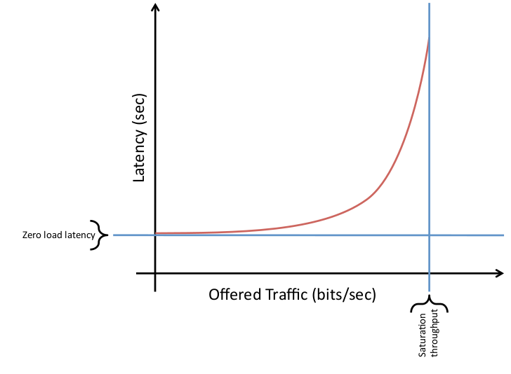
Fig1.1: Latency vs Throughput for on-chip network
Chapter 2. Interface with System Architecture
Shared memory networks in chip multiprocessors
- Shared memory and a partitioned global address space (PGAS)
- With the shared-memory model, communication occurs implicitly through the loading and storing of data and the accessing of instructions. As a result, the shared-memory model is an intuitive way to realize this sharing.
- Two key characteristics due to mem hierarchy for shared memory :
- the cache coherence protocol that makes sure nodes receive the correct up-to-date copy of a cache line, and
- the cache hierarchy.
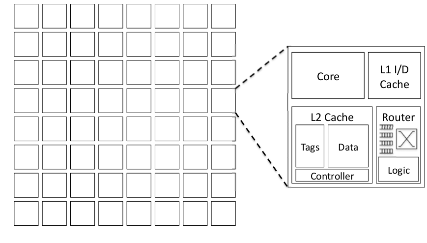
Fig2.1: Shared Memory Chip Multiprocessors Arhictecture
Impact of coherence protocol on network performance
- Any number of nodes may cache a copy of memory to read from; if a node wishes to write to that memory address, it must ensure that no other nodes are caching that address.
- Broadcast protocol: coherence request are sent to all nodes
- One interconnect for ordering and a higher bandwidth
- Unordered interconnect for data transfers
- Diectory protocal: point-to-point messages
- Type of message : (1) Unicast (2) Multicast (3) Broadcast
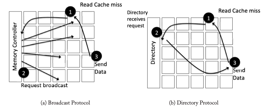
Fig2.2: Coherence protocol network request examples
Protocol-level network deadlocks
- Network needs to be free from protocol-level deadlock
- If both processors generate a burst of requests tha fill the network resources, both processors will be stalled waiting for remote replies before they can consume additional outstanding requests. If replies utilize the same network resources as requests, those replies cannot make forward progress resulting in deadlock.
- Mutliple virtual channels can be used to prevent deadlock.(See Chapter 5) In short, use different virtual channels for different message classes => the cyclic dependence between requests and responses is broken in the networks.
- Three typical classes:
- Requests: loads, stores, upgrades, writebacks
- Intervensions: messages sent from directory to request modified data be transferred to a new node
- Responses: invalidataion acknowledgements, negative acknowledgements, data messages
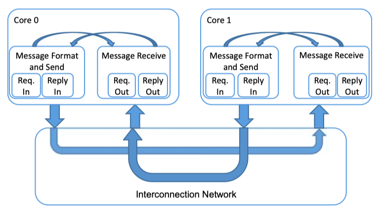
Fig2.3: Coherence protocol network request examples
Impact of cache hierarchy implementation
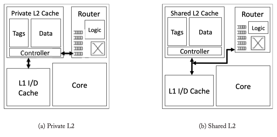
Fig2.4: Private and Shared Caches
- Private vs Shared L2 Caches : With a private L2 cache, ‘L1 miss’ will only be sent to the local L2 cache. Then, the reqeust could hit, or be forwarded to a remote L2 cache that hold its directory, or access to off-chip memory. On the otherhand, with shared L2 cache, L1 miss will be sent to an L2 bannk determined by the miss address (not necessarily the local L2 bank).
- Drawback of private cache: (1) Need to replicate data, and (2) increased L2 miss rate.
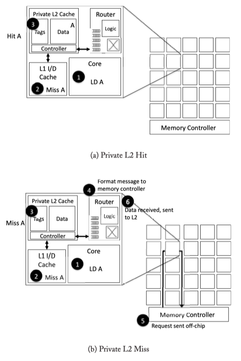
Fig2.5: Private L2 caches walk-through example. (a) Private L2 Hit case. (b) Private L2 miss case. Then, the load of A misses in the private L2 cache and must be sent to the network interface(4), sent through the network to the memory controller (5), sent off-chip and finally re-traverse the network back to the the requestor (6)
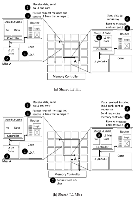
Fig2.6: Shared L2 cache walk-through example. (a) Private L2 Hit case. If L1 misses, the router will format the request message and send it to the one of the remote shared nodes. if the shared L2 hit, the date will be sent to the requsetor. (b) If shared L2 cache in a remote node misses, the remote node will generate request for data to the off-chip memory, and send the acquired date to the original requestor
Home node and memory controller design issues
Home node : With a directory protocol, each address statically maps to a home node. The directory information resides at the home node which is responsible for ordering requests to all addresses that map to this home node.The directory either supplies the data from off-chip, either from memory or from another socket, or sends intervention messages on-chip to acquire data and/or permissions for the coherence request. For a shared L2 cache, the home node with directory information is the cache bank that the address maps to. From the example in Figure 2.6, the directory is located at the tile marked A for address A. If remote L1 cache copies need to be invalidated (for a write request to A), the directory will send those requests through the network. With a private L2 cache configuration, there does not need to be a one-to-one correspondence between the number of home nodes and the number of tiles. Every tile can house a portion of the directory (n home nodes), there can be a single centralized directory, or there can be a number of home nodes in between 1 and n. Broadcast protocols such as the Opteron protocol [41] require an ordering point similar to a home node from which to initiate the broadcast request.
Memory controller: Handle the data request from the network to memory outside the chip.
 Fig2.7: Memory controller inside/outside the core
Miss and transaction status holding registers
- Processor-to-Network interface is responsible fro formatting network messages to handle cache misses (due to a load or store), cache line permission upgrads, and cache line evictions.
- MSHR: Miss status handling register
- cache miss => MSHR => send message to the network
recieve message from the network => MSHR matching => complete cache miss actions.
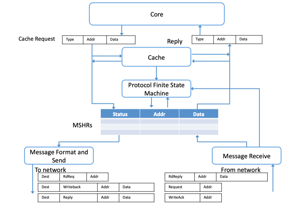
Fig2.8: Processor-to-Network Interface (adapted from Dally and Towles [47])- Memory-to-Network interface is responsible for receiving memory request messages from processors (caches) and initiating replies.
- TSHR: Transaction status handling registers
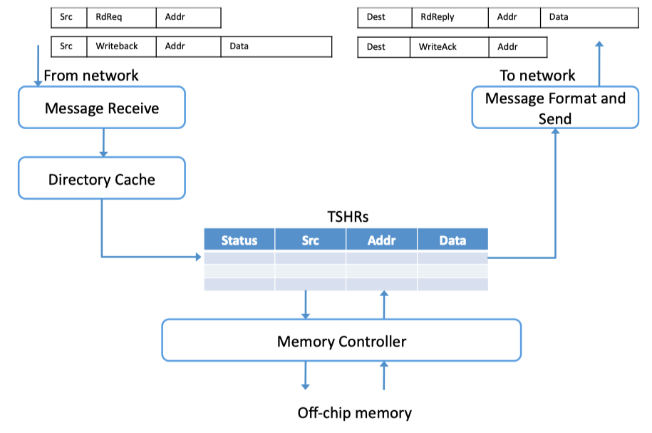
Fig2.9: Memory-to-Network Interface (adapted from Dally and Towles [47])
Synthesized NOCs in MPSOCs
- Holy grail in NoC design in MPSoCs is to allow designers to feed in NoC traffic characterziation to a design tool, which will then automaticallly generate a fully sythesizable NoC design
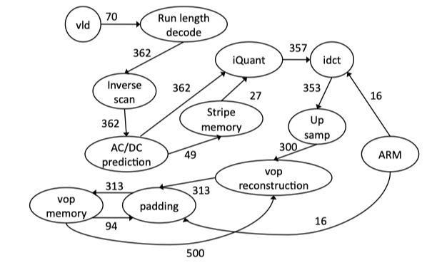
Fig2.10: VOPD (video decoder) task graph example from [104, 30]. The peak/average communication bandwidth between cores are characterized and marked on the links between cores
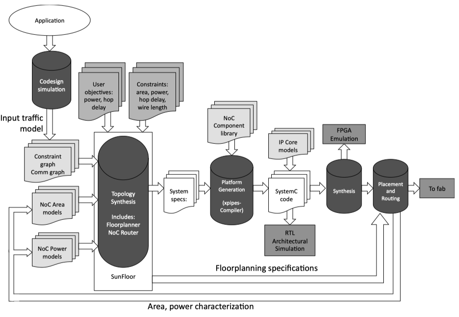
Fig2.11: Synthesis flow from [183]
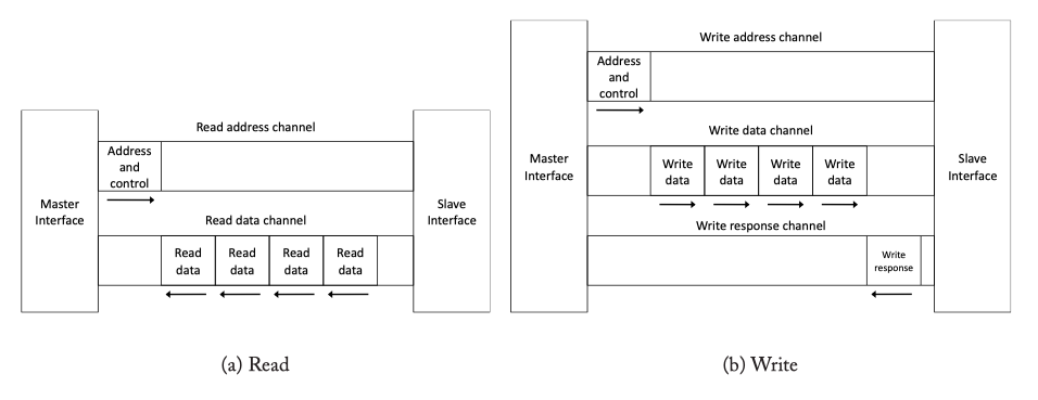
Fig2.13: AXI read (addresss, data) and write (address, data, response) channel
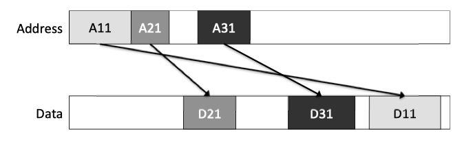
Fig2.14: The AXI Protocol allows messages to complete out of order: D21 returns data prior to D11 even though A11 occurred prior to A21.
Chapter 3. Topology
- The on-chip network topology determines the physical layout and connections between nodes and channels in the network.
- The implementation complexity cost of a topology depends on two factors: the number of links at each node (node degree) and the ease of laying out a topology on a chip (wire lengths and the number of metal layers required).
Metrics for comparing Topologies
- Question: How to compare the characteristics of different topologies?
- Bisection bandwidth: a metric for off-chip networks. Not proper for NoC because of large number of wires in NoC.
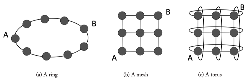
Fig3.1: Common on-chip network topologies.
- Degree a topology : ~ the number of ports at routers. e.g. ring = 2, torus = 4, mesh = 2~4 (not uniform)
- Hop count : ~ network latency
- Maximum channel load : maximum number of bits per second (bps) that can be injected by every node into the network before it saturates
Path diversity : A topology that provides multiple shortest paths ( R_(src−dst) > 1, where R represents the path diversity) between a given source and destination pair has greater path diversity than a topology where there is only a single path between a source and destination pair ( R_(src−dst) = 1).
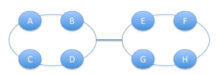
Fig3.2: Channel load example with 2 rings connected via a single channel. The max channel load for the bottleneck channel = 4 = 8x1/2
Direct Topologies
- Ring : Rings fall into the torus family of network topologies as k-ary 1-cubes.
- Mesh : Mesh and torus networks can be described as k-ary n-cubes , where k is the number of nodes along each dimension, and n is the number of dimensions.
- Tori : With a torus, all nodes have the same degree
Indirect Topologies
- BUTTERFLIES : Butterfly networks can be described as k-ary n-flies. Such a network would consist of k^n terminal nodes (e.g.cores,memory),and comprises n stages of k^(n−1) k×k intermediate switch nodes. The primary disadvantages of a butterfly network are the lack of path diversity and the inability of these networks to exploit locality. (Poor for unbalanced traffic patterns)
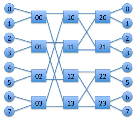
Fig3.3: A 2-ary 3-fly butterfly network.
- CLOS NETWORKS : a three-stage network characterized by the triple, (m,n,r) where m is the number of middle stage switches, n is the number of input/output ports on each input/output switch (first and last stage switches), and r is the number of first/last stage switches. When m > (2n−1), a Clos network is strictly non-blocking. A disadvantage of a Clos network is its inability to exploit locality between source and destination pairs.
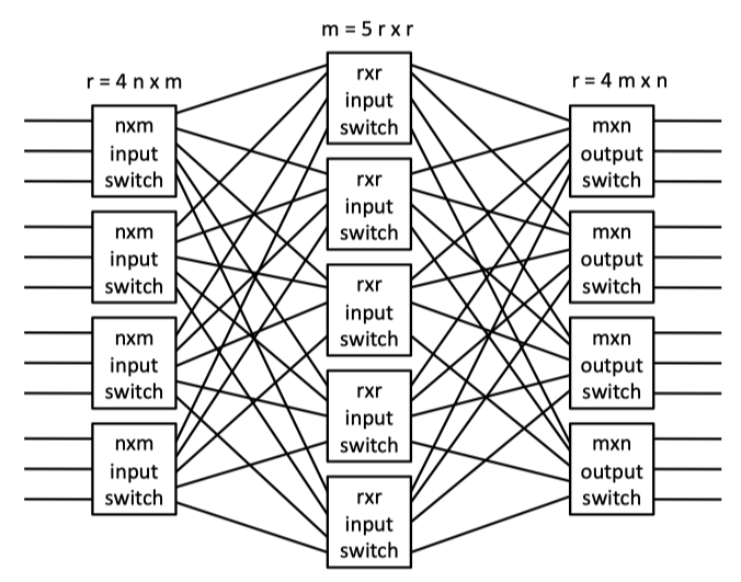
Fig3.4: An (m = 5, n = 3, r = 4) symmetric Clos network with r = 4n × m input-stage switches, m = 5r × r middle-stage switches, and r = 4m × n output-stage switches. Crossbars form all switches.
- FAT TREES : a binary tree network in which wiring resources increase for stages closer to the root node (Figure 3.5a). A fat tree can be constructed from a folded Clos network, as shown in Figure 3.5b giving path diversity over the tree network in Figure 3.5a.
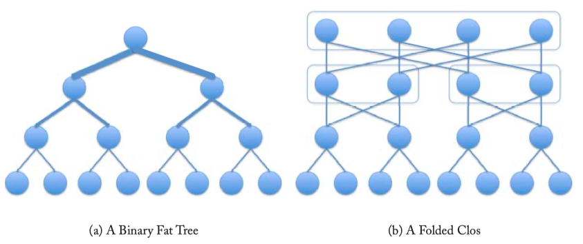
Fig3.5: A fat tree network. (b) A Clos network can be folded along the middle set of switches so that the input and output switches are shared. A 5-stage folded Clos network characterized by the triple (2, 2, 4) is depicted. The center stage is realized with another 3-stage Clos formed using (2, 2, 2) Clos network. This Clos network is folded along the top row of switches.
Irregular topologies
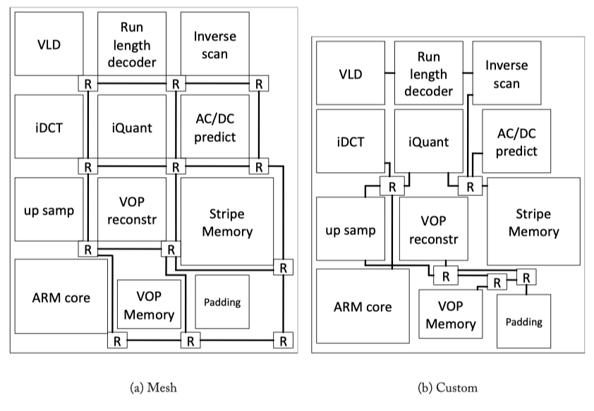
Fig3.6: A regular (mesh) topology and a custom topology for a video object plane decoder (VOPD) (from [30]).
- Splitting: With splitting, a large crossbar connecting all nodes is first created and then iteratively split into multiple small switches to accommodate a set of design constraints.
- Merging: Alternatively, a network with a larger number of switches such as a mesh or torus can be used as a starting point. From this starting point, switches are merged together to reduce area and power.
Topology Synthesis Algorithm Example
Finding optimal topology? An NP-hard problem! -> several heuristics have been proposed to find the best topology in an efficient manner like…
The min-cut partition is performed so that the edges of the graph that cross partitions have lower weights than the edges within partitions. Additionally, the number of nodes assigned to each partition remains nearly the same. Such a min-cut partition will ensure that traffic flows with high bandwidth will use the same switch for communication.
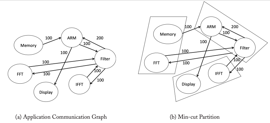
Fig3.7: Topology Synthesis Algorithm example.
Layout and Implementation
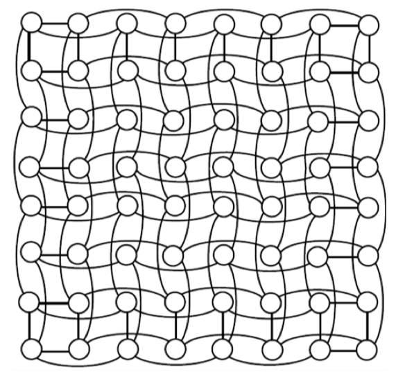
Fig3.8: Layout of a 8x8 folded torus.
Concentrator
- Up to this point, we have assumed a one-to-one correspondence between network nodes and terminal nodes. However, this need not be the case. Frequently, multiple cores that do not require the bandwidth of a single network node will share a node by using concentrators.
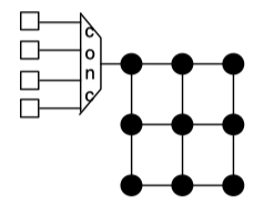
Fig3.9: A mesh where four nodes are sharing bandwidth through a concentrator.
Implication of abstract metrics on on-chip implementation
- High node degree : high port count, additional input buffer queue(s), additional requestors to the allocators, additional ports to the crossbar switch, (= all major contributors to a router’s critical path delay, area footprint, and power).
- Link complexity depends on the link width, as link area and power overheads correlate more closely with the number of wires than the number of ports.
- Hop count : Overall network latency and power. However, hop count does not always correlate with network latency in practice, as it depends heavily on the router pipeline length and the link propagation delay.
- For instance, a network with only 2 hops, router pipeline depths of 5 cycles, and long inter-router distances requiring 4 cycles for link traversal, will have an actual network latency of 18 cycles.
- Conversely, a network with 3 hops where each router has a single-cycle pipeline and the link delay is a single cycle, will have a total network latency of only 6 cycles.
- However, unfortunately, factors such as router pipeline depth are typically not known until later in the design cycle.
- Maximum channel load : A good proxy for network saturation throughput (congestion) and maximum power. Since it is a good proxy for saturation, it is also very useful for estimating peak power, as dynamic power is highest with peak switching activity and utilization in the network.
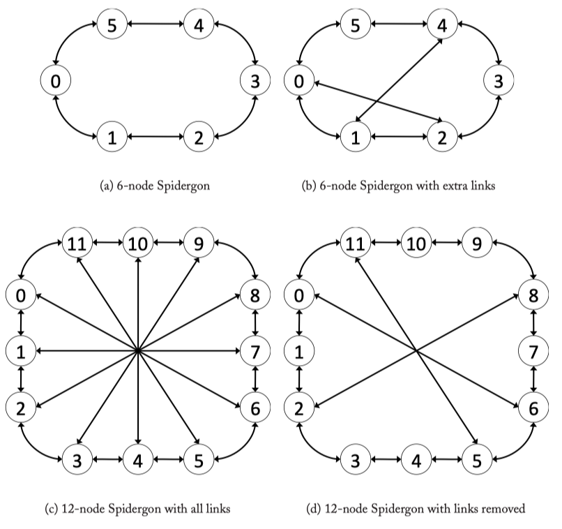
Fig3.10: Various Spidergon Topologies.
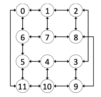
Fig3.11: 12 Node Full Spidergon Layout for the logical Spidergon depicted in Figure 3.10c.
Chapter 4. Routing
- The goal of the routing algorithm is to distribute traffic evenly among the paths supplied by the network topology, so as to avoid hotspots and minimize contention,thus improving network latency and throughput.
TYPES OF ROUTING ALGORITHMS
- Three classes:
- deterministic: dimension-ordered routing (DOR)
- oblivious : randomly choose path
- adaptive : the path depends on network traffic situation
- Other two classes:
- minimal
- non-minimal
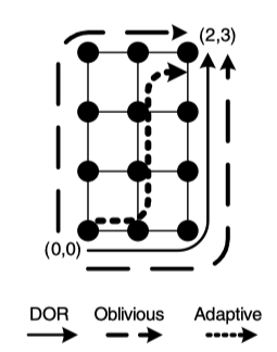
Figure 4.1: DOR illustrates an X-Y route from (0,0) to (2,3) in a mesh, while Oblivious shows two alternative routes (X-Y and Y-X) between the same source-destination pair that can be chosen obliviously prior to message transmission. Adaptive shows a possible adaptive route that branches away from the X-Y route if congestion is encountered at (1,0)
DEADLOCK AVOIDANCE
- A deadlock occurs when a cycle exists among the paths of multiple messages
- Deadlock freedom can be ensured in the routing algorithm by preventing cycles among the routes generated by the algorithm, or in the flow control protocol by preventing router buffers from being acquired and held in a cyclic manner
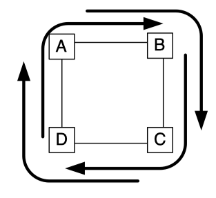
Figure 4.2: A classic network deadlock where four packets cannot make forward progress as they are waiting for links that other packets are holding on to.
DETERMINISTIC DIMENSION-ORDERED ROUTING
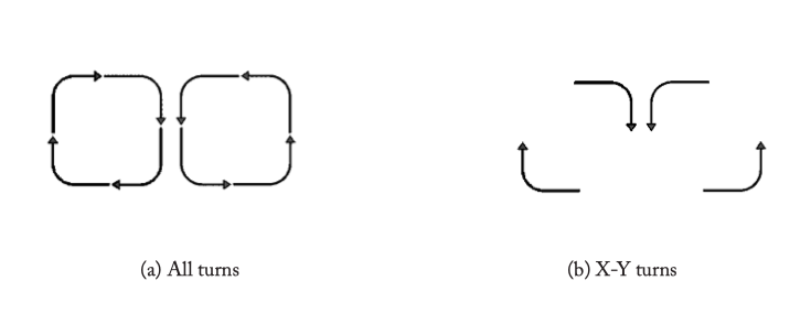
Figure 4.3: Possible routing turns for a 2D Mesh.
OBLIVIOUS ROUTING
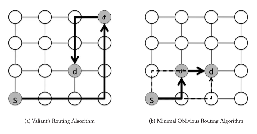
Figure 4.4: Oblivious Routing Examples.
ADAPTIVE ROUTING
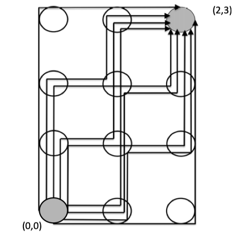
Figure 4.5: Adaptive Routing Example.
- If adaptive routing allows misrouting -> Livelock -> limit the maximum number of misroutes.
ADAPTIVE TURN MODEL ROUTING
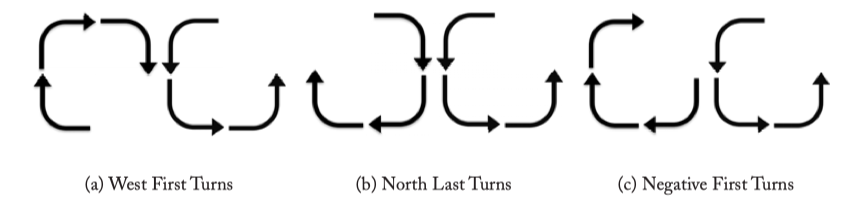
Figure 4.6: Turn Model Routing.
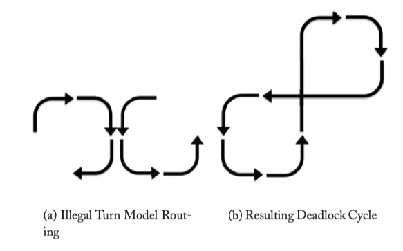
Figure 4.7: Turn Model Deadlock.
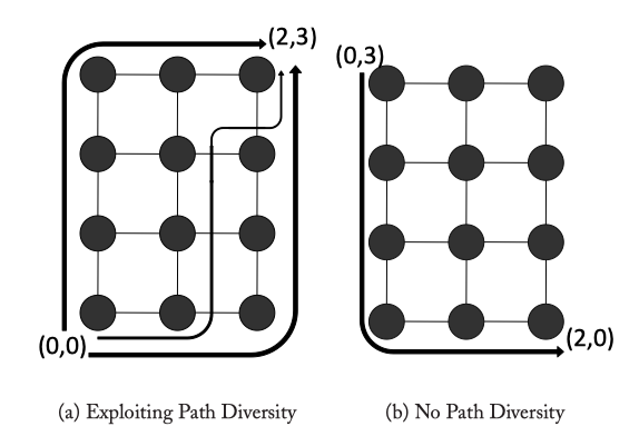
Figure 4.8: Negative-First Routing example.
IMPLEMENTATION
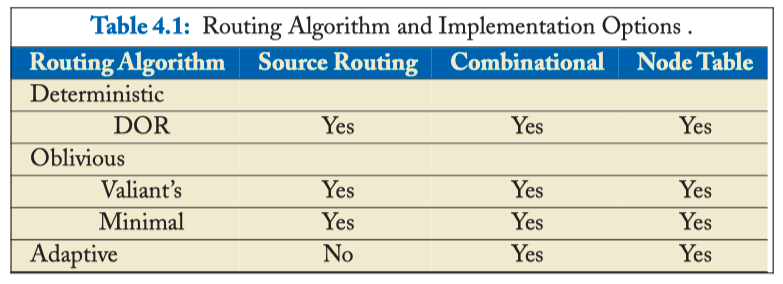
Table 4.1: Routing Algorithm and Implementation Options .
SOURCE ROUTING
- The route can be embedded in the packet header at the source, known as source routing. For instance, the X-Y route in Figure 4.1 can be encoded as < E, E, N, N, N, Eject >, while the Y-X route can be encoded as < N, N, N, E, E, Eject >. At each hop, the router will read the leftmost direction off the route header, send the packet towards the specified outgoing link, and strip off the portion of the header corresponding to the current hop.
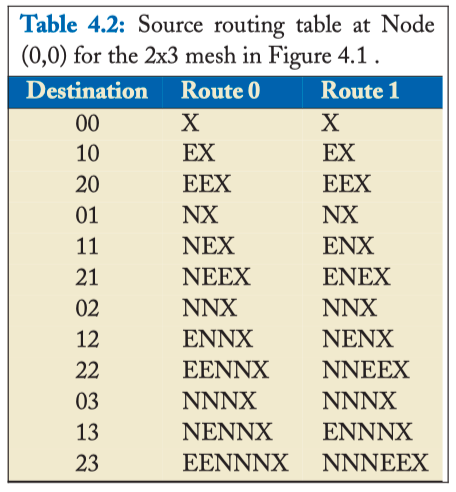
Table 4.2: Source routing table at Node (0,0) for the 2x3 mesh in Figure 4.1
NODE TABLE-BASED ROUTING
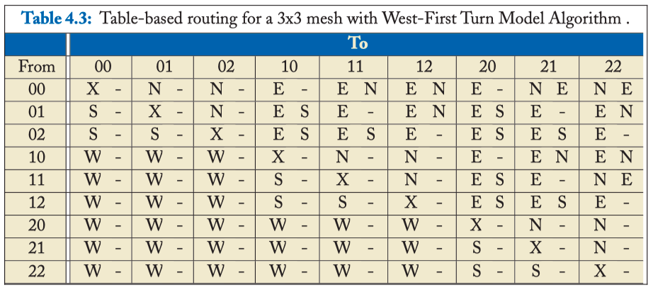
Table 4.3: Table-based routing for a 3x3 mesh with West-First Turn Model Algorithm
COMBINATIONAL CIRCUITS
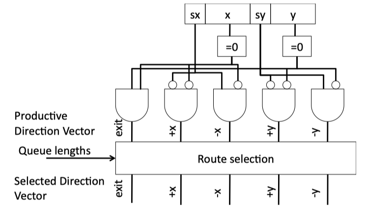
Figure 4.9: Combinational Routing Circuit for 2-D Mesh.
ADAPTIVE ROUTING
- Route adjustments can be implemented by modifying the header,by employing combinational circuitry that accepts as input these congestion signals, or by updating entries in a routing table.
ROUTING ON IRREGULAR TOPOLOGIES
- Common routing implementations for irregular networks rely on source table routing or node-table routing
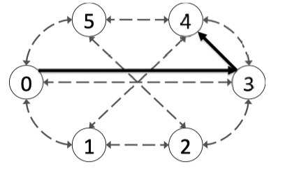
Figure 4.10: A 6 node Spidergon with the highlighted path from Node 0 to Node 4 using the Across-
Chapter 5. Flow Control
- Flow control governs the allocation of network buffers and links. It determines when buffers and links are assigned to messages, the granularity at which they are allocated, and how these resources are shared among the many messages using the network.
MESSAGES, PACKETS, FLITS, AND PHITS
- Message -> Packets -> Flits -> Phits
- Head/Body/Tail filts contain cache line & cache coherence command
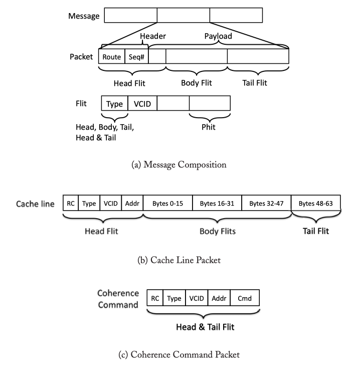
Figure 5.1: Composition of Message, Packets, Flits: Assuming 16-byte wide flits and 64-byte cache lines, a cache line packet will be composed of 5 flits and a coherence command will be a single-flit packet. The sequence number (Seq#) is used to match incoming replies with outstanding requests, or to ensure ordering and detect lost packets.
MESSAGE-BASED FLOW CONTROL
- Circuit switching pre-allocates resources (links) across multiple hops to the entire message.
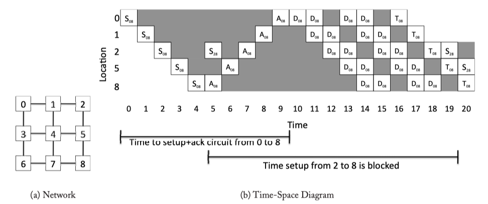
Figure 5.2: Circuit-switching example from Core 0 to Core 8, with Core 2 being stalled. S: Setup flit, A: Acknowledgement flit,D: Data message,T:Tail (deallocation) flit.Each D represents a message; multiple messages can be sent on a single circuit before it is deallocated. In cycles 12 and 16, the source node has no data to send.
PACKET-BASED FLOW CONTROL
- Packet-based flow control techniques first break down messages into packets, then interleave these packets on the links, thus improving link utilization. Unlike circuit switching, the remaining techniques will require per-node bufferin to store in-flight packets.
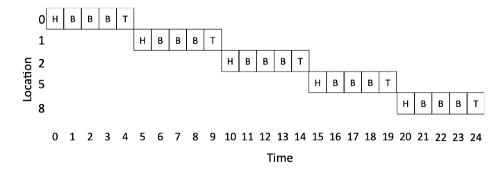
Figure 5.3: Store and Forward Example.
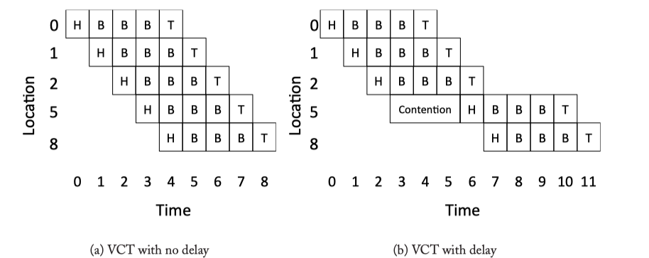
Figure 5.4: Virtual Cut Through Example.
FLIT-BASED FLOW CONTROL
- To reduce the buffering requirements of packet-based techniques, flit-based flow control mechanisms exist. Low buffering requirements help routers meet tight area or power constraints on-chip.
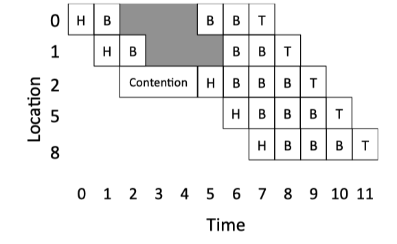
Figure 5.5: Wormhole Example.
VIRTUAL CHANNELS
- Virtual channels have been explained as the “swiss-army knife” of interconnection networks
- Essentially, a virtual channel (VC) is basically a separate queue in the router; multiple VCs share the physical wires (physical link) between two routers. By associating multiple separate queues with each input port, head-of-line blocking can be reduced. Virtual channels arbitrate for physical link bandwidth on a cycle-by-cycle basis.
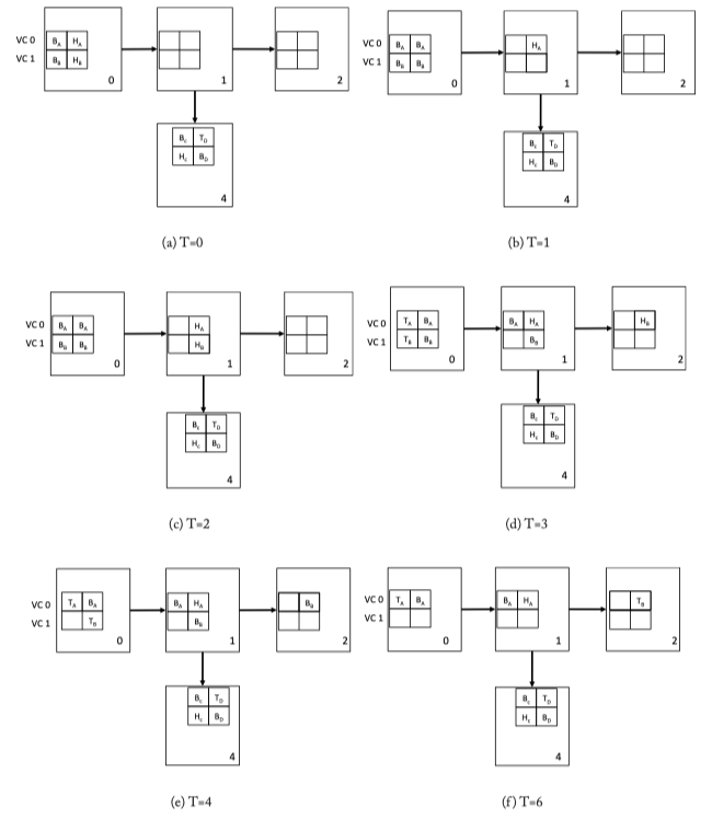
Figure 5.6: Virtual Channel Flow Control Walk-through Example. Two packets A and B are broken into 4 flits each (H: head, B: Body, T: Tail).

Table 5.1: Summary of flow control techniques.
DEADLOCK-FREE FLOW CONTROL
- DATELINE AND VC PARTITIONING, ESCAPE VCS, BUBBLE FLOW CONTROL
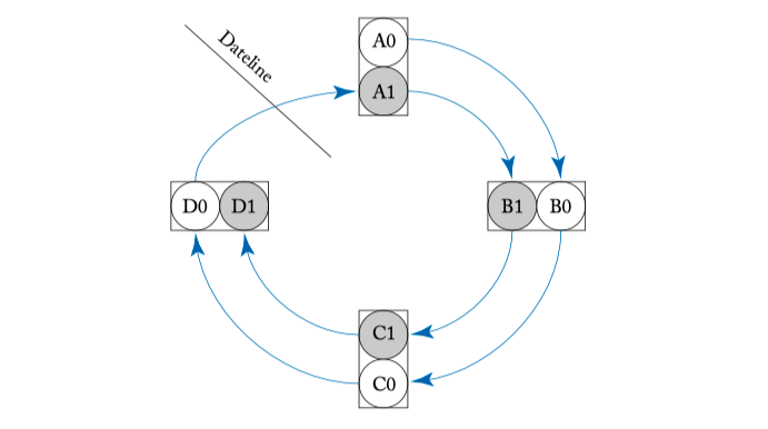
Figure 5.7: Two virtual channels with separate buffer queues denote with white and grey circles at each router are used to break the cyclic route deadlock in Figure 4.2.
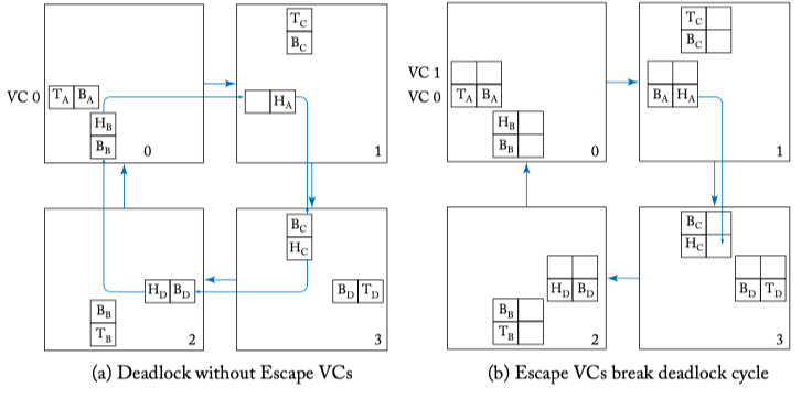
Figure 5.8: Escape virtual channel example. Virtual Channel 1 serves as an escape virtual channel that is dimension order XY routed.
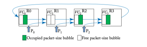
Figure 5.9: Bubble flow control example.
BUFFER BACKPRESSURE
- As most on-chip network designs cannot tolerate the dropping of packets, there must be buffer backpressure mechanisms for stalling flits. Flits must not be transmitted when the next hop will not have buffers available to house them.
- Credit-based, On/off signal
IMPLEMENTATION
- BUFFER SIZING FOR TURNAROUND TIME
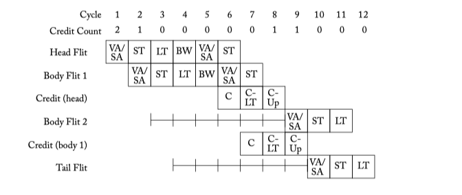
Figure 5.10: Throttling due to too few buffers. Flit pipeline stages discussed in Chapter 6. C: Credit send. C-LT: Credit link traversal. C-Up: Credit update.
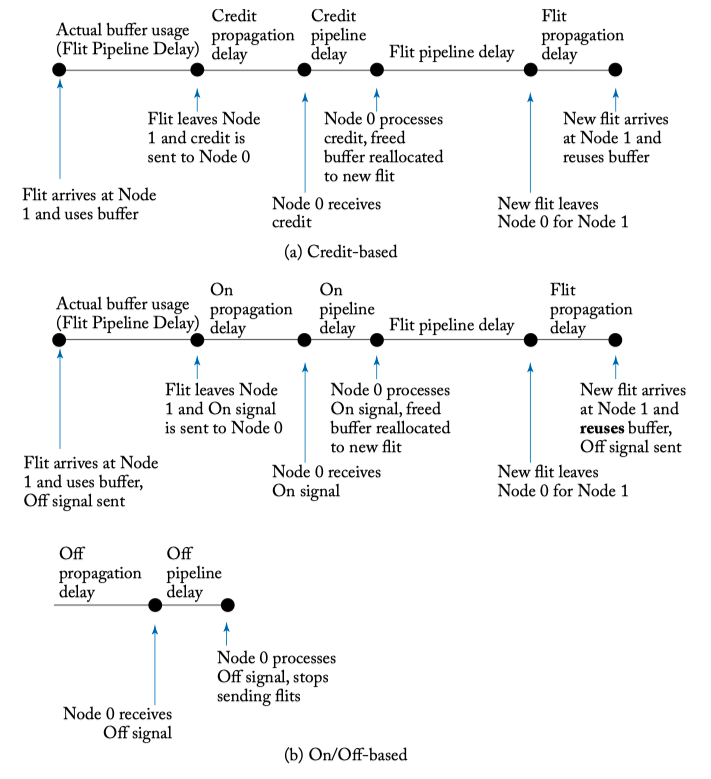
Figure 5.11: Buffer backpressure mechanisms time lines.
- REVERSE SIGNALING WIRES
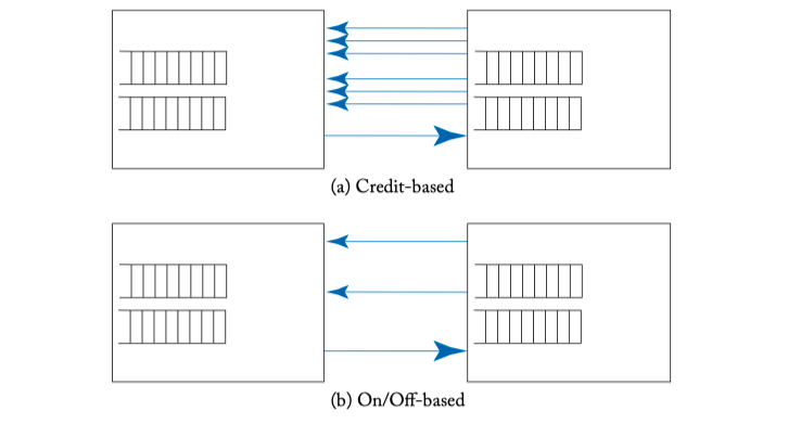
Figure 5.12: Reverse signaling overhead.
Chapter 6. Router Microarchitecture
VIRTUAL CHANNEL ROUTER MICROARCHITECTURE
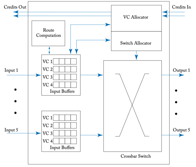
Figure 6.1: A credit-based virtual channel router microarchitecture.
BUFFERS AND VIRTUAL CHANNELS
- Buffer organization
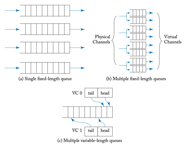
Figure 6.2: Buffer and VC organizations.
- Input VC state: Global, Rount, Output VC, Credit Count, Pointers
SWITCH DESIGN
The crossbar switch of a router is the heart of the router datapath. It switches bits from input ports to output ports, performing the essence of a router’s function.
Crossbar design
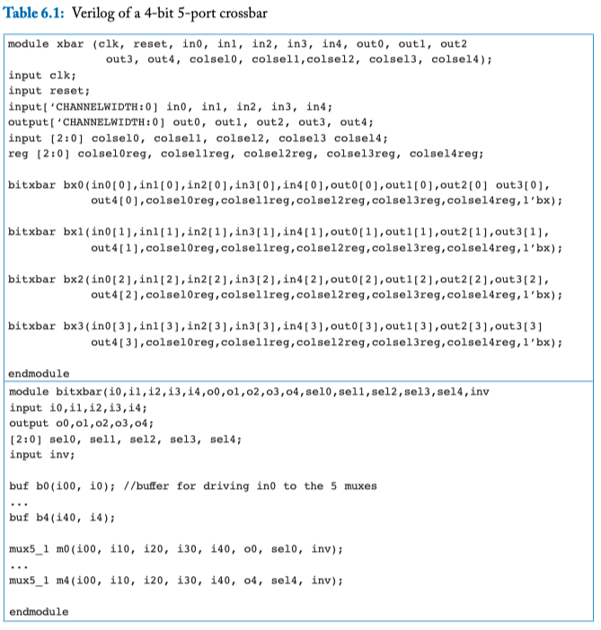
Table 6.1: Verilog of a 4-bit 5-port crossbar
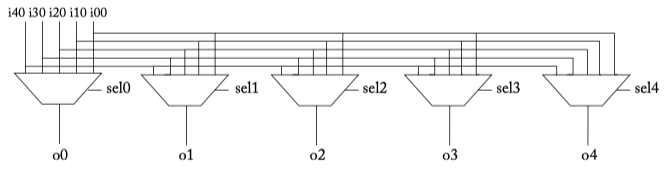
Figure 6.3: Crossbar composed of many multiplexers.
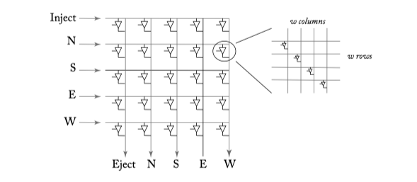
Figure6.4: A 5x5 crosspoint crossbar switch. Each horizontal and vertical line is w bits wide (1 phit width). The bold lines show a connection activated from the south input port to the east output port.
- Crossbar speedup
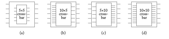
Figure 6.5: Crossbars with different speedups for a 5-port router. (a) No crossbar speedup, (b) crossbar with input speedup of 2, (c) crossbar with output speedup of 2, and (d) crossbar with input and output speedup of 2.
- Crossbar slicing
ALLOCATORS AND ARBITERS
- Round-robin arbiter
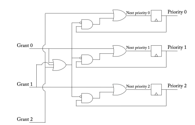
Figure 6.6: Round-robin arbiter.
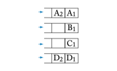
Figure 6.7: Request queues for arbiter examples.
- Matrix arbiter
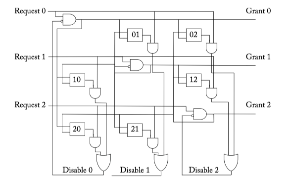
Figure 6.8: Matrix arbiter. The boxes w_ij represent priority bits. When bit w_ij is set, request i has a higher priority than request j .
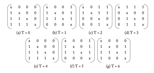
Figure 6.9: Matrix arbiter priority update for the request stream from Figure 6.7.
- Separable allocator
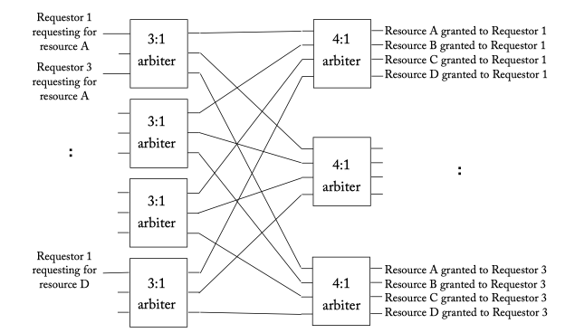
Figure 6.10: A separable 3:4 allocator (3 requestors, 4 resources) which consists of four 3:1 arbiters in the first stage and three 4:1 arbiters in the second. The 3:1 arbiters in the first stage decides which of the 3 requestors win a specific resource, while the 4:1 arbiters in the second stage ensure a requestor is granted just 1 of the 4 resources.
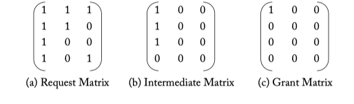
Figure 6.11: Separable allocator example.
- Wavefront allocator
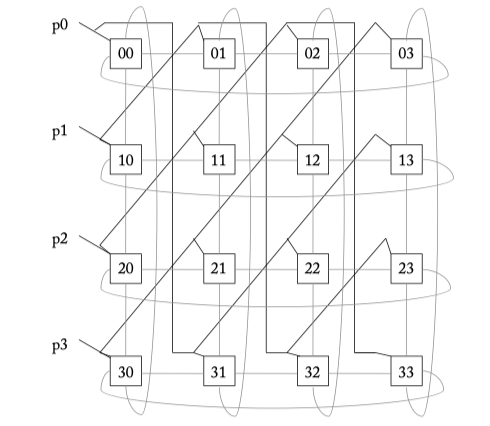
Figure 6.12: A 4 x 4 wavefront allocator. Diagonal priority groups are connected with bold lines. Connections for passing tokens are shown with grey lines.
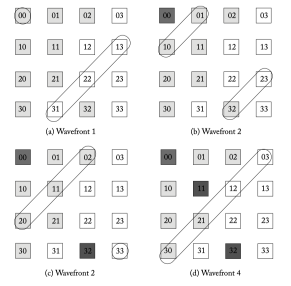
Figure 6.13: Wavefront allocator example.
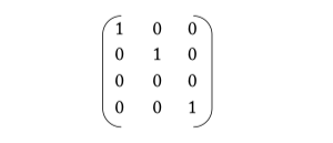
Figure 6.14: Wavefront grant matrix.
- Allocator Organization
PIPELINE
- A head flit, upon arriving at an input port, is first decoded and buffered according to its input VC in the buffer write (BW) pipeline stage. Next, the routing logic performs route computation (RC) to determine the output port for the packet. The header then arbitrates for a VC corresponding to its output port (i.e., the VC at the next router’s input port) in the VC allocation (VA) stage. Upon successful allocation of a VC, the header flit proceeds to the switch allocation (SA) stage where it arbitrates for the switch input and output ports. On winning the output port, the flit is then read from the buffer and proceeds to the switch traversal (ST) stage, where it traverses the crossbar. Finally, the flit is passed to the next node in the link traversal (LT) stage. Body and tail flits follow a similar pipeline except that they do not go through RC and VA stages, instead inheriting the route and the VC allocated by the head flit. The tail flit, on leaving the router, deallocates the VC reserved by the head flit.
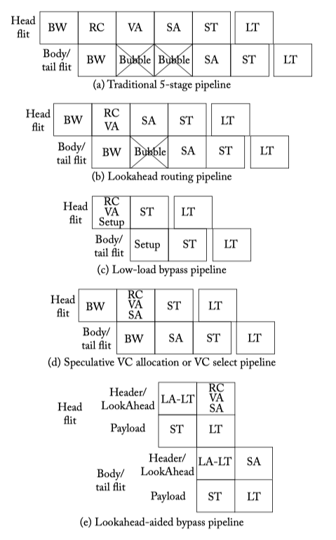
Figure 6.15: Router pipeline [BW: Buffer Write, RC: Route Computation, VA: Virtual Channel Allocation, SA: Switch Allocation, ST: Switch Traversal, LT: Link Traversal].
- Pipeline optimization:
- Lookahead Routing = Next route comput = Route pre-computation
- Low-load bypassing
- Speculative VA
- VC selection
- Lookahead bypass
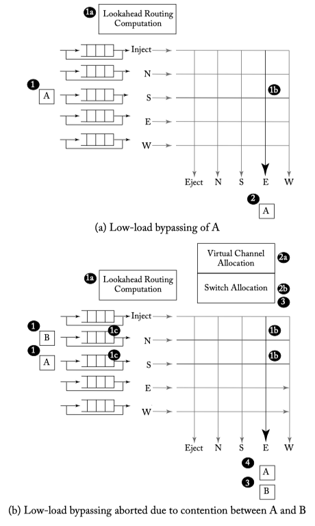
Figure 6.16: Low-load bypass example.
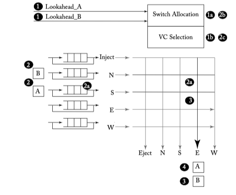
Figure 6.17: Lookahead bypass example—Lookahead_B wins and B bypasses, A gets buffered.
LOW-POWER MICROARCHITECTURE
- Dynamic power vs leakage power
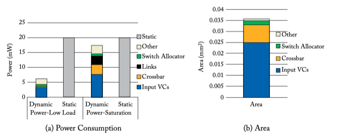
Figure 6.18: Power and area of a 1-cycle mesh router at 32 nm [64].
PHYSICAL IMPLEMENTATION
- Router floorplanning
- Buffer implementation
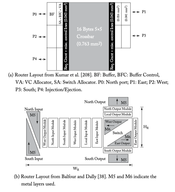
Figure 6.19: Two router floorplans.